This page was generated from getting_started/tutorial.ipynb.
Tutorial
This is a brief tutorial of basic Metagraph usage.
First, we import Metagraph:
import metagraph as mg
Inspecting Types and Available Algorithms
The default resolver automatically pulls in all registered Metagraph plugins.
The default resolver also links itself with the metagraph namespace, allowing users to ignore the default resolver in most cases.
res = mg.resolver
A hierarchy of available types is automatically added as properties on res.
dir(res.types)
['BipartiteGraph',
 'DataFrame',
 'EdgeMap',
 'EdgeSet',
 'Graph',
 'Matrix',
 'NodeMap',
 'NodeSet',
 'Vector']
Alternatively, simply access the types directly from mg.
Most attributes of res are exposed as attributes on mg for convenience.
dir(mg.types)
['BipartiteGraph',
 'DataFrame',
 'EdgeMap',
 'EdgeSet',
 'Graph',
 'Matrix',
 'NodeMap',
 'NodeSet',
 'Vector']
Two important concepts in Metagraph are abstract types and concrete types.
Abstract types describe a generic kind of data container with potentially many equivalent representations.
Concrete types describe a specific data object which fits under the abstract type category.
One can think of abstract types as data container specifications and concrete types as implementations of those specifications.
For each abstract type, there are several concrete types.
Within a single abstract type, all concrete types are able to represent equivalent data, but in a different format or data structure.
Here we show the concrete types which represent Graphs:
dir(mg.types.Graph)
['GrblasGraphType', 'NetworkXGraphType', 'ScipyGraphType']
Available algorithms are listed under mg.algos and grouped by categories.
Note that these are also available under res.algos.
dir(mg.algos)
['bipartite',
 'centrality',
 'clustering',
 'embedding',
 'flow',
 'subgraph',
 'traversal',
 'util']
dir(mg.algos.traversal)
['all_pairs_shortest_paths',
 'astar_search',
 'bellman_ford',
 'bfs_iter',
 'bfs_tree',
 'dfs_iter',
 'dfs_tree',
 'dijkstra',
 'minimum_spanning_tree']
Example Usage
Let’s see how to use Metagraph by first constructing a graph from an edge list.
Begin with an input csv file representing an edge list and weights.
data = """
Source,Destination,Weight
0,1,4
0,3,2
0,4,7
1,3,3
1,4,5
2,4,5
2,5,2
2,6,8
3,4,1
4,7,4
5,6,4
5,7,6
"""
Read in the csv file and convert to a Pandas DataFrame.
import pandas as pd
import io
csv_file = io.StringIO(data)
df = pd.read_csv(csv_file)
This DataFrame represents a graph’s edges, but Metagraph doesn’t know that yet. To use the DataFrame within Metagraph, we first need to convert it into an EdgeMap.
A PandasEdgeMap takes a DataFrame plus the labels of the columns representing source, destination, and weight. With these, Metagraph will know how to interpret the DataFrame as an EdgeMap.
em = mg.wrappers.EdgeMap.PandasEdgeMap(df, 'Source', 'Destination', 'Weight', is_directed=False)
em.value
| Source | Destination | Weight | |
|---|---|---|---|
| 0 | 0 | 1 | 4 |
| 1 | 0 | 3 | 2 |
| 2 | 0 | 4 | 7 |
| 3 | 1 | 3 | 3 |
| 4 | 1 | 4 | 5 |
| 5 | 2 | 4 | 5 |
| 6 | 2 | 5 | 2 |
| 7 | 2 | 6 | 8 |
| 8 | 3 | 4 | 1 |
| 9 | 4 | 7 | 4 |
| 10 | 5 | 6 | 4 |
| 11 | 5 | 7 | 6 |
Convert EdgeMap to a Graph
Graphs and EdgeMaps have many similarities, but Graphs are more powerful. Graphs can have weights on the nodes, not just on the edges. Graphs can also have isolate nodes (nodes with no edges), which EdgeMaps cannot have.
Most Metagraph algorithms take a Graph as input, so we will convert our PandasEdgeMap into a Graph. In this case, it will become a NetworkXGraph.
g = mg.algos.util.graph.build(em)
g
<metagraph.plugins.networkx.types.NetworkXGraph at 0x7fcd30f17850>
g.value.edges(data=True)
EdgeDataView([(0, 1, {'weight': 4}), (0, 3, {'weight': 2}), (0, 4, {'weight': 7}), (1, 3, {'weight': 3}), (1, 4, {'weight': 5}), (3, 4, {'weight': 1}), (4, 2, {'weight': 5}), (4, 7, {'weight': 4}), (2, 5, {'weight': 2}), (2, 6, {'weight': 8}), (5, 6, {'weight': 4}), (5, 7, {'weight': 6})])
Translate to other Graph formats
Because Metagraph knows how to interpret g as a Graph, we can easily convert it other Graph formats.
Let’s convert it to a ScipyGraph. This format stores the edges and weights in a scipy.sparse matrix along with a numpy array mapping the position to a NodeId (in case the nodes are not sequential from 0..n). Any node weights are stored in a separate numpy array.
g2 = mg.translate(g, mg.wrappers.Graph.ScipyGraph)
g2
<metagraph.plugins.scipy.types.ScipyGraph at 0x7fcd30f2c750>
The matrix is accessed using g2.value. The node list is accessed using .node_list.
We can verify the weighs and edges by inspecting the sparse adjacency matrix directly.
g2.value.toarray()
array([[0, 4, 0, 2, 7, 0, 0, 0],
       [4, 0, 0, 3, 5, 0, 0, 0],
       [0, 0, 0, 0, 5, 2, 8, 0],
       [2, 3, 0, 0, 1, 0, 0, 0],
       [7, 5, 5, 1, 0, 0, 0, 4],
       [0, 0, 2, 0, 0, 0, 4, 6],
       [0, 0, 8, 0, 0, 4, 0, 0],
       [0, 0, 0, 0, 4, 6, 0, 0]], dtype=int64)
We can also convert g into an adjacency matrix representation using a GrblasGraph. This also stores the edges and node weights separately.
g3 = mg.translate(g, mg.types.Graph.GrblasGraphType)
g3
<metagraph.plugins.graphblas.types.GrblasGraph at 0x7fcd30f40650>
g3.value
M0
grblas.Matrix
nvals
nrows
ncols
dtype
24
8
8
INT64
grblas.Matrix |
nvals |
nrows |
ncols |
dtype |
| 24 | 8 | 8 | INT64 |
| 0 | 1 | 2 | 3 | 4 | 5 | 6 | 7 | |
|---|---|---|---|---|---|---|---|---|
| 0 | 4 | 2 | 7 | |||||
| 1 | 4 | 3 | 5 | |||||
| 2 | 5 | 2 | 8 | |||||
| 3 | 2 | 3 | 1 | |||||
| 4 | 7 | 5 | 5 | 1 | 4 | |||
| 5 | 2 | 4 | 6 | |||||
| 6 | 8 | 4 | ||||||
| 7 | 4 | 6 |
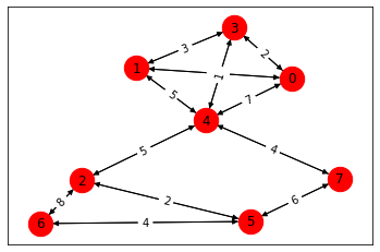
We can also visualize the graph.
import grblas
grblas.io.draw(g3.value)
Inspect the steps required for translations
Rather than actually converting g into other formats, let’s ask Metagraph how it will do the conversion. Each conversion requires a translator (written by plugin developers) to convert between the two formats. However, even if there isn’t a direct translator between two formats, Metagraph will find a path and take several translation steps as needed to perform the task.
The mechanism for viewing the plan is to invoke the translation from mg.plan.translate rather than mg.translate. Other than the additional .plan, the call signature is identical.
In this first example, there is a direct function which translates between NetworkXGraphType and ScipyGraphType.
mg.plan.translate(g, mg.types.Graph.ScipyGraphType)
[Direct Translation]
NetworkXGraphType -> ScipyGraphType
In this next example, there is no direct function which convert NetworkXGraphType into a GrblasGraphType. Instead, we have to first convert to ScipyGraphType and then to GrblasGraphType before finally arriving at our desired format.
While Metagraph will do the conversion automatically, understanding the steps involved helps users plan for expected computation time and memory usage. If needed, plugin developers can write a plugin to provide a direct translation path.
mg.plan.translate(g, mg.types.Graph.GrblasGraphType)
[Multi-step Translation]
(start)  NetworkXGraphType
           -> ScipyGraphType
 (end)       -> GrblasGraphType
Algorithm Example #1: Breadth First Search
Algorithms are described initially in an abstract definition. For bfs_iter, we take a Graph and return a Vector indicating the NodeIDs in the order visited.
After the abstract definition is written, multiple concrete implementations are written to operate on concrete types.
Let’s look at the signature and specific implementations available for bfs_iter.
mg.algos.traversal.bfs_iter.signatures
Signature:
        (graph: Graph({}), source_node: NodeID, depth_limit: int = -1) -> Vector({})
Implementations:
        (graph: ScipyGraphType({}), source_node: NodeID, depth_limit: int = -1) -> NumpyVectorType({})
        (graph: NetworkXGraphType({}), source_node: NodeID, depth_limit: int = -1) -> NumpyVectorType({})
We see that there are two implementations available, each with a different type of input graph.
Let’s perform a breadth-first search with our different representations of g. We should get approximately the same answer no matter which implementation is chosen (same NodeIDs within each depth level of the traversal).
cc = mg.algos.traversal.bfs_iter(g, 0)
cc
array([0, 1, 3, 4, 2, 7, 5, 6])
cc2 = mg.algos.traversal.bfs_iter(g2, 0)
cc2
array([0, 1, 3, 4, 2, 7, 5, 6])
Similar to how we can view the plan for translations, we can view the plan for algorithms.
No translation is needed because we already have a concrete implementation which takes a NetworkXGraph as input.
mg.plan.algos.traversal.bfs_iter(g, 0)
nx_breadth_first_search_iter
(graph: NetworkXGraphType({}), source_node: NodeID, depth_limit: int = -1) -> NumpyVectorType({})
=====================
Argument Translations
---------------------
** graph **
NetworkXGraphType
** source_node **
NodeID
** depth_limit **
int
---------------------
In the next example, g2 also satisfies a concrete implementation, so no input translation is required.
mg.plan.algos.traversal.bfs_iter(g2, 0)
ss_breadth_first_search_iter
(graph: ScipyGraphType({}), source_node: NodeID, depth_limit: int = -1) -> NumpyVectorType({})
=====================
Argument Translations
---------------------
** graph **
ScipyGraphType
** source_node **
NodeID
** depth_limit **
int
---------------------
Algorithm Example #2: Pagerank
Let’s look at the same pieces of information, but for pagerank. Pagerank takes a Graph and returns a NodeMap indicating the rank value of each node in the graph.
First, let’s verify the signature and the implementations available.
We see that there are two implementations available, taking a NetworkXGraph or GrblasGraph as input.
mg.algos.centrality.pagerank.signatures
Signature:
        (graph: Graph({'edge_type': 'map', 'edge_dtype': ('float', 'int')}), damping: float = 0.85, maxiter: int = 50, tolerance: float = 1e-05) -> NodeMap({})
Implementations:
        (graph: NetworkXGraphType({}), damping: float = 0.85, maxiter: int = 50, tolerance: float = 1e-05) -> PythonNodeMapType({})
        (graph: GrblasGraphType({}), damping: float = 0.85, maxiter: int = 50, tolerance: float = 1e-05) -> GrblasNodeMapType({})
Let’s look at the steps required in the plan if we start with a ScipyGraph. Then let’s perform the computation.
We see that the ScipyGraph will need to be translated to a GrblasGraph in order to call the algorithm. Metagraph will do this for us automatically.
mg.plan.algos.centrality.pagerank(g2)
grblas_pagerank
(graph: GrblasGraphType({}), damping: float = 0.85, maxiter: int = 50, tolerance: float = 1e-05) -> GrblasNodeMapType({})
=====================
Argument Translations
---------------------
** graph **  [Direct Translation]
ScipyGraphType -> GrblasGraphType
** damping **
float
** maxiter **
int
** tolerance **
float
---------------------
pr = mg.algos.centrality.pagerank(g2)
pr
<metagraph.plugins.graphblas.types.GrblasNodeMap at 0x7fcd32c1cd90>
The result is a GrblasNodeMap which can be inspected by looking at the underlying .value.
pr.value
v4
grblas.Vector
nvals
size
dtype
8
8
FP64
grblas.Vector |
nvals |
size |
dtype |
| 8 | 8 | FP64 |
| 0 | 1 | 2 | 3 | 4 | 5 | 6 | 7 | |
|---|---|---|---|---|---|---|---|---|
| 0.11991 | 0.11991 | 0.129191 | 0.11991 | 0.195384 | 0.133008 | 0.093041 | 0.089646 |
Let’s translate it to a numpy array.
pr_array = mg.translate(pr, mg.types.NodeMap.NumpyNodeMapType)
pr_array.value
array([0.11990989, 0.11990989, 0.12919109, 0.11990989, 0.19538403,
       0.13300793, 0.09304149, 0.08964579])
Helpful tip: The translation type can also be specified as a string
mg.translate(pr, "NumpyNodeMap")
<metagraph.plugins.numpy.types.NumpyNodeMap at 0x7fcd30ea4490>
Now let’s verify that we get the same answer with the NetworkX implementation of Pagerank. We can ensure the NetworkX implementation is called by passing in a NetworkXGraph. Because no translations are required, it will choose that implementation.
The result is a PythonNodeMapType, which is simply a Python dict.
pr2 = mg.algos.centrality.pagerank(g)
pr2
{0: 0.11990989117844908,
 1: 0.11990989117844908,
 3: 0.11990989117844908,
 4: 0.1953840289789895,
 2: 0.12919108800740858,
 5: 0.13300793197881575,
 6: 0.09304148578762082,
 7: 0.08964579171181795}
Translate to a numpy array and verify the same results (within tolerance)
pr2_array = mg.translate(pr2, "NumpyNodeMap")
pr2_array.value
array([0.11990989, 0.11990989, 0.12919109, 0.11990989, 0.19538403,
       0.13300793, 0.09304149, 0.08964579])
abs(pr2_array - pr_array.value) < 1e-15
array([ True, True, True, True, True, True, True, True])